
Note
Go to the end to download the full example code.
Read and plot maps with MadcubaMap#
Introduction to using madcubapy to read and plot FITS maps.
Usually, we would open and FITS files in python using astropy and plot them
using matplotlib. This tutorial shows how this can be done with madcubapy,
which uses the previous packages to do all the work, but in a more concise
manner, simplifying this process for the user.
We start by importing the necessary libraries for this tutorial.
from madcubapy.io import MadcubaMap
from madcubapy.visualization import add_wcs_axes
from madcubapy.visualization import add_manual_wcs_axes
from madcubapy.visualization import insert_colorbar
import matplotlib.pyplot as plt
Reading the FITS map#
When MADCUBA exports a FITS map it also creates a
history file with the same name of the FITS file ended
with _hist.csv. With the MadcubaMap class we can open these
FITS files alongside their history tables.
We can read the FITS file with the
MadcubaMap.read() method, and the
corresponding history file will be loaded as well if
present.
madcuba_map = MadcubaMap.read(
    "../examples/data/IRAS16293_SO_2-1_moment0_madcuba.fits")
Note
Due to how MADCUBA saves some FITS header cards, several astropy
warnings can pop up when reading FITS files. Usually these warnings are
unexpected card names using non-standard conventions.
The MadcubaMap class resembles the CCDData
class from Astropy with data, header, wcs, and unit
attributes, with the addition of a hist attribute, the history table
containing all the information from the history file:
madcuba_map.hist
As a failsafe, a CCDData object is also present inside the
MadcubaMap object in the ccddata attribute.
This way, we can do anything a CCDData object can with
madcubapy through this attribute.
Plotting the FITS map#
To plot FITS maps we can use the buiilt-in visualization functions of
madcubapy, or the classical option: plotting the data array with
matplotlib (and astropy for coordinates).
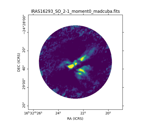
The add_wcs_axes()
method of madcubapy lets the user plot a
MadcubaMap or CCDData
quickly using only two statements.
A Figure must be set before calling
add_wcs_axes(), and it
must be the first input parameter of the function. The second mandatory
parameter is fitsmap, the map object to plot, which can be a
MadcubaMap or CCDData.
Addionally, the user can set a series of kwargs parameters, which
are passed to matplotlib.pyplot.imshow(), like vmin or
vmax, for example.
We can very quickly add a colorbar using
add_colorbar() or
insert_colorbar().
Check the Colorbar page to know more about how
these two functions work.
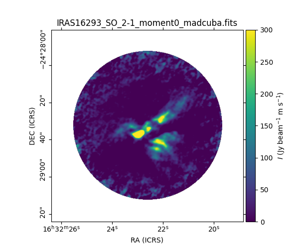
The visualization functions of madcubapy automatically parse
information from the FITS header like the units for the data.
The same figure is recreated in Method #2 using the functions of
matplotlib and astropy that madcubapy uses under the hood.
Note
For this tutorial we are calling this function using the parameter
names explicitly (i.e add_wcs_axes(fig=fig_object,
fitsmap=map_object)), and not by using positional arguments.
If one opts to use positional arguments, to quickly plot one map
the call to the function should be
add_wcs_axes(fig_object, 1, 1, 1, map_object).
This is due to the functionality of
add_wcs_axes() and its manual
version add_manual_wcs_axes()
to plot several maps in one figure. This is explained thoroughly in
Plotting image with coordinates.
The classical option: plotting the data array of the FITS files using
using matplotlib and astropy.
We can first plot the data array without bothering with any
coordinate system with the
matplotlib function imshow(), and add the
title, axis labels and a colorbar using other matplotlib functions.
Keep in mind that usually we need to do some slicing to get rid of the spectral and polarization axes if present.
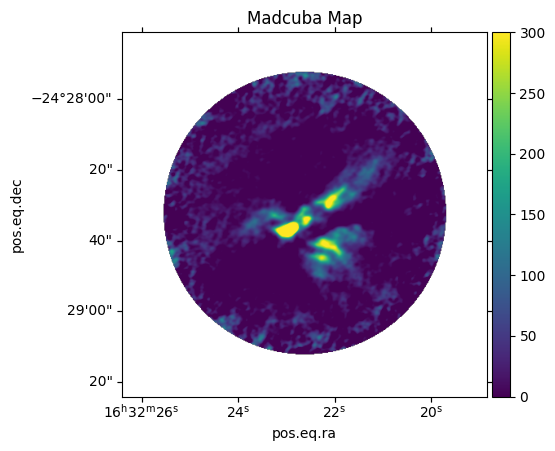
# Create a figure and plot the image
fig, ax = plt.subplots(1, 1, figsize=(6, 6))
map_data = madcuba_map.data[0, 0, :, :]  # apply slicing
img = ax.imshow(map_data, cmap='viridis', origin='lower', vmin=0, vmax=300)

# Add a colorbar
fig.colorbar(img)

# Set axis labels and title
ax.set_title('Madcuba Map')
ax.set_xlabel('X axis')
ax.set_ylabel('Y axis')

plt.show()
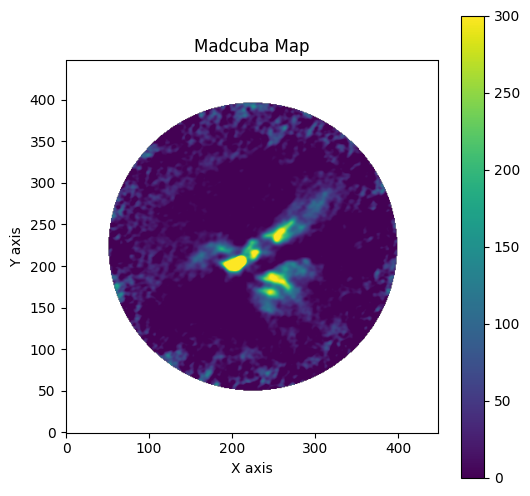
This figure uses pixel coordinates for the X and Y axes, and the colorbar does not have the same height as the image, resulting in an ugly astronomical map.
We can correct the placement of the colorbar by manually creating a new axes with the size of the image, and use it for the colorbar.
# New imports needed to create the colorbar
import matplotlib.axes as maxes
from mpl_toolkits.axes_grid1 import make_axes_locatable

# Create a figure and plot the image
fig, ax = plt.subplots(1, 1, figsize=(6, 5))
map_data = madcuba_map.data[0, 0, :, :]  # apply slicing
img = ax.imshow(map_data, cmap='viridis', origin='lower', vmin=0, vmax=300)

# Add a colorbar with the same height as the image
divider = make_axes_locatable(ax)
cax = divider.append_axes("right", size="5%", pad=0.08, axes_class=maxes.Axes)
fig.colorbar(img, cax=cax)

# Set axis labels and title
ax.set_title('Madcuba Map')
ax.set_xlabel('X axis')
ax.set_ylabel('Y axis')

plt.show()
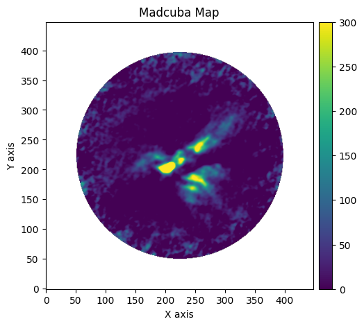
The colorbar is correctly placed, but we still have pixel coordinates.
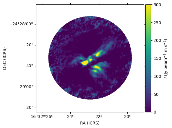
We can use Astropy to create the plot using the WCS coordinates from the FITS file.
# Create a figure and add a subplot with WCS projection
fig = plt.figure(figsize=(5, 5))
ax = fig.add_subplot(1, 1, 1, projection=madcuba_map.wcs.celestial)
map_data = madcuba_map.data[0, 0, :, :]  # apply slicing
img = ax.imshow(map_data, cmap='viridis', origin='lower', vmin=0, vmax=300)

# Add a colorbar with the same height as the image
divider = make_axes_locatable(ax)
cax = divider.append_axes("right", size="5%", pad=0.05, axes_class=maxes.Axes)
cbar = fig.colorbar(img, cax=cax, orientation='vertical')

# Set title
ax.set_title('Madcuba Map')

plt.show()
As we can see, astropy created a
WCSAxes object and set the X and Y
labels to the correct values read from the FITS file, but their
representation looks kind of ugly, and we still do not have a label for
the colorbar. We must set the labels manually, and we have to look into
the FITS header to get the units of the data, located in the BUNIT
card.
For this FITS file, the units of the data are \({\rm Jy \ beam^{-1} \ m \ s^{-1}}\). We can set the labels with:
# Set correct labels
ax.coords[0].set_axislabel("RA (ICRS)")
ax.coords[1].set_axislabel("DEC (ICRS)")
cbar.set_label(r'$I \ {\rm (Jy \ beam^{-1} \ m \ s^{-1})}$')
Fix units#
Some programs export the BUNIT fits card incorrectly with more than one slash
and astropy has problems parsing the units from those strings. The
MadcubaMap.fix_units() method
tries to fix this problem and correctly parse the units.
For example, CARTA exports units like this. When we read a CARTA map,
madcubapy warns us that no history file has been found,
which we can ignore when working with FITS files not created by MADCUBA.
carta_map = MadcubaMap.read("../examples/data/IRAS16293_SO2c_moment0_carta.fits")
WARNING: Default history file not found.
If we check the units of the map we can see that they are incorrect,
because the BUNIT card has a string with multiple slashes: ‘Jy/beam.km/s’.
When astropy tries to parse this, it incorrectly places the
\({\rm km}\) on the denominator:
print(f"Astropy parsed unit: {carta_map.unit}")
print(f"FITS header BUNIT: {carta_map.header["BUNIT"]}")
Astropy parsed unit: Jy / (beam km s)
FITS header BUNIT: Jy/beam.km/s
We can run the
MadcubaMap.fix_units() method
of the MadcubaMap object to fix this. It is important to note that the
CCDData object inside MadcubaMap
also gets the correct units when they are fixed.
carta_map.fix_units()

print(f"MadcubaMap unit: {carta_map.unit}")
print(f"CCDData unit: {carta_map.ccddata.unit}")
MadcubaMap unit: Jy km / (beam s)
CCDData unit: Jy km / (beam s)
Even though a CARTA exported map does not have a _hist.csv file, it is
encouraged to read it as a MadcubaMap, even when the user wants to work with
a CCDData object if some functionality isn’t working with a
MadcubaMap object.
This is the reason why we have the failsafe CCDData object
in the MadcubaMap.ccddata attribute.
We can work with it just as if it was an object directly read with the
CCDData.read() method from astropy
(because it actually is read this way).
Total running time of the script: (0 minutes 1.080 seconds)